Wind River is proud to announce a new member of the commercially supported Wind River Linux family, the Wind River Linux Distro. The Wind River Linux Distro (Distro) is a binary Linux distribution created from our source-code based Linux product.
Wind River Systems, the leader in the IoT and embedded operating systems, has long provided customers with the ability to create their own purpose-built Linux operating system from source. Wind River starts with the Yocto Project and adds a significant amount of integration with semiconductor vendor SDKs to provide a commercially supportable Linux distribution builder for intelligent edge solution developers.
Wind River Linux is used in tens of thousands of telecommunications, industrial, aerospace and defense, and automotive embedded solutions, but we realized that not all customers need the flexibility of building and Linux operating system from source code.
Introducing the binary Distro
The Distro is intended for intelligent edge solution developers who want to leverage the tremendous investment in embedded device hardware and open-source software made by Wind River but want to avoid the time and effort of building Linux from source.
The Distro provides multiple methods for solution developers to create a purpose-built Linux OS from binary images. These methods include: micro-start self-deploying images, Linux Assembly Tool (LAT), dnf package feeds, a container base image on Dockerhub, and a software development kit (SDK).
Because bug fixes and security updates are important for security and stability, the Distro provides OSTree updates that can be used to deliver fixes or even upgrade images to a new release. Solution developers can create their own images, containers, packages & package feeds, and even their own OSTree update feeds.
Hardware support
One of the key advantages of using Wind River Linux has been the support for a wide variety of hardware platforms. Wind River takes the SDKs from semiconductor vendors and integrates them into the Wind River Linux Yocto Project source base. Unlike some other binary distributions, the Wind River Linux Distro is not limited to just upstream Linux hardware enablement and we regularly update our hardware support from the latest semiconductor vendor SDK.
The Wind River Linux Distro has been available for several X86 and Arm hardware platforms as a free and unsupported download since 2021. Thousands of images have been downloaded since we made the images available with the launch of Wind River Linux LTS21 last year.
With this announcement, we are now offering commercial support for some of the Distro hardware platforms.
Like the Wind River Linux source-based product, the Wind River Linux Distro does not require any paid subscriptions or royalties on deployed systems: the Wind River Linux Distro is sold on a per-project basis.
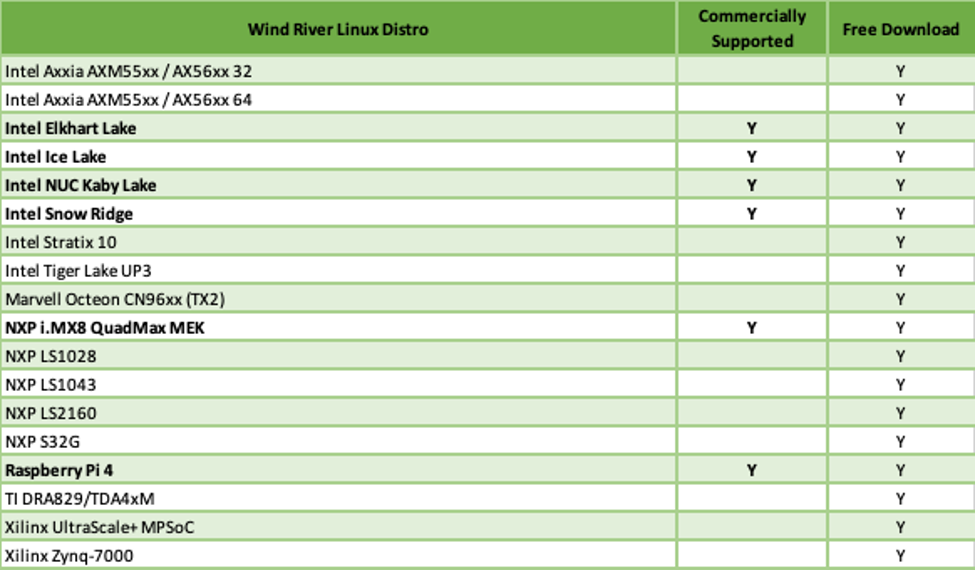
Wind River Linux Distro hardware
We will add commercial support for additional hardware platforms based on customer demand.
Choosing the “Right” Wind River Linux
Generally, the Wind River Linux source-based product provides the ultimate amount of flexibility and reproducibility and is particularly well suited to intelligent edge solution developers who require complex customization of Linux including the kernel.
In contrast, the Wind River Linux Distro is the best choice for rapid prototyping and deployment when there is limited need for Linux kernel customization and generally requires significantly less resources than our Yocto Project based source product.
Choosing between Wind River Linux and Wind River Linux Distro
Try it out for free
Anyone can try the Distro for free. Just go to https://www.windriver.com/products/linux/download. After registering and choosing your hardware platform, you will be sent a link to the images and SDK.
The quick start guide Distro Developers Guide can help you to use Distro tools such as the Linux Assembly Tool (LAT) and how to build your embedded solution on top of the Wind River Linux Distro.
Summary
The Wind River Linux Distro is a true binary distribution of Linux that solution developers can use to quickly provide a Linux OS foundation for their intelligent edge solution. Solution developers can try out the free version of the Distro knowing that commercial support is available when they deploy their solution.
Wind River Linux is not a traditional Linux distro, but is a complete Linux development platform for embedded device development. It comes with the latest LTS kernel, toolchains, tools, and more than 500 packages enabling customers to develop a wide variety of devices across networking, A&D, industrial, and consumer industries. Customers can use Wind River Linux to produce a supported, customized Linux OS that exactly meets the requirements for their embedded application.
Wind River Linux is based on the open-source Yocto Project and Wind River is one of the leading contributors to that community. Wind River Linux provides application portability and ease of integration. It also enables increased ease of use with the layered architecture that allows developers to simply swap out a Board Support Package (BSP) for another one and easily build images for multiple hardware platforms. This simplifies creation of embedded Linux images for deployment in 5G network infrastructure, automotive, industrial, and other applications.
Wind River uses a DevOps approach to develop LTS21 using continuous integration (CI) and continuous delivery (CD) infrastructure and processes.
Key features of LTS 21 include:
Based on Linux LTS 5.10 Kernel and the Yocto Project 3.3
The Linux Assembly Tool which can be used to perform a number of tasks to help manage your images, such as building and publishing RPM packages, generating images from package feeds for specific hardware, and generating an updated SDK. In addition, you can add or remove packages, and specify any pre- and post-build instructions for the build, which lets you customize your image to meet your needs.
Wind River Linux now supports the Qt 5 toolkit version 5.15.2 to provide the tools necessary to get QT-based applications running on your Wind River Linux system image.
TensorFlow machine learning that simplifies the creation of a system image that employs machine learning to develop and test applications.
OpenVINO (coming in lTS 21 RCPL 1) enables Convolutional Neural Networks (CNNs) to extend Intel® hardware to provide high-performance AI and deep learning inference capabilities.
chrony, a replacement for NTP that can work well when external time references are only intermittently accessible.
gcc and the toolchain is upgraded to version 10.2.x
Enhanced OSTree support allows image upgrades on deployed devices and creation of images from an existing system.
Full enablement for the Wind River Workbench including Visual Studio code support that provides a complete suite of developer tools to allow you to quickly configure your operating system, analyze and tune your software, and debug an entire system.
Pre-built binary distribution that allows for dramatically faster prototyping of embedded systems Linux OS by eliminating the need to build the entire OS from source. With the Linux Assembly Tool, the binary distribution allows creation of a customized embedded OS in as little as an hour, compare to more than a day when using the source -based Wind River Linux solution.
Hardware support in LTS21 includes:
o Intel Axxia AXM55xx / AXM56xx
o Intel Stratix 10
o Intel x86 Tiger Lake (Core)
o Intel x86 Ice Lake-SP (Xeon)
o Intel NUC7i5BNH (Kaby Lake)
o Intel Snow Ridge (Atom Server)
o Marvell Armada CN96xx
o NXP i.MX7
o NXP i.MX8 QM
o NXP QorIQ LS1028A
o NXP S32G EVB/RDB2
o Raspberry Pi 4 Model B
o TI TDA4
o Xilinx Zynq UltraScale+ MPSoC
o Xilinx Zynq-7000
Additional hardware support is planned for delivery in future Rolling Cumulative Patch Layer (RCPL) updates to LTS 21
Wind River LTS releases are supported for up to five years under the normal support agreements, with additional support available beyond five years with the legacy support offering.
LTS 21 provides new capabilities for SoC providers and OHVs to create their own customized embedded Linux OS that are supported by Wind River. For more information about LTS 21, see the documentation at
This was one of the first questions the cable support rep asked me when I called to report slow Internet speeds.
Like everybody else, I am conducting almost all my activities over the Internet these days. So when I noticed my network speed slowing to a crawl, I immediately did a few diagnostic tasks like rebooting my cable modem. When that didn’t help, I gritted my teeth and called support at Spectrum Cable. After passing through the VRU gauntlet (don’t get me started!) I finally got to a support rep that asked me that question. The problem is, I didn’t really have any idea when my network bandwidth started to deteriorate.
What was worse is that the problem was intermittent so even when I thought it was “fixed” the problem reoccurred. Eventually the problem was resolved by swapping out my ancient cable modem, but I wanted to make sure that I was aware of network problems when they started occurring. I needed to find a way to monitor my network speed on an ongoing basis.
Searching for a solution
First attempt – Raspberry Pi
I quickly found this blog by Simon Hearne https://simonhearne.com/2020/pi-speedtest-influx/ about running speedtest on a Raspberry Pi and capturing the results in InfluxDB. This blog gave me a lot of information on the potential solution, but I had some issues with implementing it.
The first issue is that I only have one Raspberry Pi currently in “production” use, and that use is running pihole. I was concerned about the additional load of running speedtest, InfluxDB, and Grafana on the Pi. But I went ahead and installed the configuration on the Raspberry Pi.
Unfortunately, the bandwidth results I got were significantly lower and inconsistent compared to the results I was seeing from Ookla speedtest on my desktop.
I (incorrectly) hypothesized that the Raspberry Pi didn’t have enough processing capacity but that turned out not to be the cause of the discrepancy.
Finding a new host
I started looking around for another system in my house that was always on and had enough processing power to support the network monitoring. I have a newish Dell laptop I purchased last year dedicated to running family Zoom meetings from my kitchen. The “Zoom” machine is running 64bit Windows 10 Home and has Core I5 processors with 8gb of RAM, so I thought it would be able to handle the monitoring workload.
Since I changed my personal desktop to a Mac four years ago, this would be a good opportunity to brush up on my Windows 10 skills. A quick search showed that InfluxDB, Grafana, and Python were all available for Windows 10.
Speedtest-cli issues
I replicated Simon’s monitoring solution on the Windows 10 machine, but quickly noticed that the network bandwidth had the same slow and inconsistent results I saw on the Raspberry Pi. Doing more digging I found that there are two speedtest command line interface (cli) implementations. The original speedtest-cli had a number of issues reporting reliable network speeds. The newer Ookla version worked much more reliably.
Unfortunately, my Python skills were not up to changing Simon Hearn’s python code to use the Ookla speedtest, so I searched for an alternative.
Speedtest based on Ookla
I found a python solution in this project https://github.com/aidengilmartin/speedtest-to-influxdb by Aiden Gilmartin. It was targeted for Linux, but I felt that I could reuse the InfluxDB and Grafana infrastructure I had already installed on the Windows 10 system. Aiden’s python script speedtest2influx.py had an additional advantage in that it was set up to run continuously at regular intervals.
It took me several days to get these tools running on Windows 10 and I wanted to pass on my learning. A lot of this time was spent re-learning Windows, particularly Windows 10.
Resource for network bandwidth monitoring on Windows 10
Resources needed
A number of different resources and tools are needed to implement network monitoring. Some are specific to Windows, but most are Windows versions of the Linux tools.
Resources
Description
Location
Windows 10 64-bit running on an X86 PC
The target Windows 10 machine should have sufficient power and memory to run the application.
Make sure you are running installation programs as an administrator
One thing I learned is that most of the installation tasks should be run as administrator.
Many of the problems I ran into were the result of using just my Admin id to install the applications needed for this project.
Some of the installation programs will default to install only for the local user, which can cause issues later when trying to run things as a service.
So always run installation programs as administrator – either by running in a Command window or PowerShell as administrator or by running the installation program from your Download directory.
I also set my User Access Control to the lowest level that still notified me about potential changes.
Installing Speedtest CLI
Since the data provided by the Ookla Speedtest is the core of this application, we can start there. Rather than install the standard GUI speedtest, we are going to install the Ookla Speedtest CLI (Command Line Interface).
Select the Open with Windows Explorer to automatically unzip the archive file.
A Windows Explorer window will open with two files, speedtest.exe and speedtest.md.
Copy the speedtest.exe file to someplace in your %PATH%
Start up a command window and test speedtest cli
If you can’t find speedtest, then the directory you copied it to is not in your %PATH%
Installing Python
I chose to install Python from https://www.python.org/downloads/windows/ but you could also use the Microsoft App store. Either way works. I chose the 64bit version. Just make sure you are installing for all users on the system and to add Python to environment variables.
You can start the Python installation from your Download location. Make sure you run the installer as an administrator
Make sure that you check the Install for All users and Add Python to environment variables options.
Be sure to enable the pip feature.
After a few moments, Python should be installed.
Start up a command window ensuring that you start it with administrator privileges and enter:
cd “\Program Files\Python38
pip install influxdb
pip show influxdb
Notice the Location: is pointing to the location where the InfluxDB package was installed. You will need that information for the next step.
Next, we are going to add the search path for Python packages to the system environment variables.
Navigate to the Windows Control Panel -> System and Security -> Systems -> Advanced Settings
Add PYTHONPATH as a System variable and point it to the location where the InfluxDB was installed in the previous step. This ensures that all Python programs running as a service can find the InfluxDB package.
Reboot after the installation to ensure the system variables are set to include the Python executables. You are now finished installing Python
Installing InfluxDB
InfluxDB is used to store the values gathered by the speedtest cli. The process for installing InfluxDB described here https://devconnected.com/how-to-install-influxdb-on-windows-in-2019/ was pretty easy to follow. I just needed to make some tweaks to make it ready for recording speedtest results.
Go to the first command window where you started influxd.exe and close the window to shut down InfluxDB.
Set up InfluxDB as a Windows Service
To run InfluxDB as a service you will need another program: NSSM (Non-Sucking Service Manager). This tool makes it easy to set up any program as a Windows service so that it will be automatically restarted with the system.
Go to https://nssm.cc/download and download the latest stable version. Use the Open in Windows Explorer option to automatically unpack the zip file.
Once the zip file is unpacked, double-click on the nssm directory and then the win64 directory to get to the nssm.exe file.
If you receive a “204 No Content” message then InfluxDB is working.
Installing the data gathering python script and other files
Set up a directory to hold the python and other files you will need, such as c:\Speedtestservice
mkdir c:\Speedtestservice
Getting speedtest2influx.py
First get the Aiden Gilmartin’s python script speedtest2influx.py from GitHub. There are lots of ways to download GitHub projects but we are just going to use the easiest method to pull a single file
You should see Aiden’s python script speedtest2influx.py
Right click on the Raw button and select Save Link as…
And save to the directory C:\Speedtestservice
Note: Different browsers have somewhat different save dialogs, but the end goal is to save the file speedtest2influx.py and get it into the directory you will run it from.
Getting speedtestservice.bat and Speedtest-jay.json
Now we will download a bat file that we will use to test the speedtest service and a json file that is the grafana console. We will get these from my GitHub repository.
Follow the previous process to download these two files into your C:\Speedtestservice directory
You need to edit two things in the bat file: the influx password DB_PASSWORD you set earlier during the installation of InfluxDB and the PYTHONPATH variable you also set earlier.
Ideally the PYTHONPATH would be obtained from the system variable you set earlier. I had several cases where the PYTHONPATH was not set when running as a service, so included it in the .bat file as insurance.
The TEST_INTERVAL variable sets the amount of time in seconds between speedtest measurements.
I am currently using 900 seconds = 15 minutes since I have been having trouble with my internet speeds. For most people, 1800 seconds/30 minutes is probably good enough. Do not set the TEST_INTERVAL to a value below 900 seconds because Ookla may block you. Remember that Ookla provides these measurements as a free service – don’t abuse it.
The PRINT_DATA=TRUE will record the speedtest results in a service log we will discuss later.
Save the file.
Now let’s test the batch file.
Open a command window and CD to the c:\Speedtestservice directory
Run the speedtestservice.bat
If you see Speedtest successful and Data written to DB successfully the testing was successful.
The speedtest will run every 15 minutes until you cancel it. Since we are only using the .bat file to test, you should terminate once you see the test has completed successfully.
Enter CTRL+C to cancel the batch execution.
Creating the speedtestservice Windows service
To ensure that the speedtest is automatically restarted when the system is restarted, we will use the NSSM tool to set up the python file speedtest2influx.py to run as a service.
As before, go to a command line window and enter
nssm install Speedtestservice
You will be putting information into multiple tabs in the NSSM gui.
Under the Application tab, you set up the parameters for the application to be run.
Path: C:\Program Files\Python38\python.exe Location of python Startup Directory: :\SpeedtestService Arguments: C:\SpeedtestService\speedtest2influx.py The application
Now press the right arrow button at the top left to go to the Details tab and set up some info that describes what this service does.
This is where you will set all the environmental variables needed for the application.
There are more variables than will fit in the window; don’t omit any!
DB_ADDRESS=127.0.0.1 DB_USER=grafana DB_PASSWORD=<put your password for influxdb here> TEST_INTERVAL=900 PRINT_DATA=TRUE PYTHONPATH=c:\users\admin\appdata\roaming\python\python38\site-packages
Finally click on the Install service button. You have used NSSW to install speedtest as a Windows service.
Open the Services application in Windows. You should see the Speedtestservice enabled, but not running.
Click Start to start the Speedtestservice service
You should see the service start and move to “Running” state. If you see it stop or say “Paused”, you have a problem. Use the log files in the C:\Speedtestservice folder to diagnose the problem. The two problems I saw were problems opening the InfluxDB package in python (PYTHONPATH should fix this) and an invalid user/password for InfluxDB.
Assuming the service is started and running, you are now automatically collecting the speedtest results every 15 minutes and storing the data into the InfluxDB database speedtest_db .
The final step is to install and configure grafana to display the data.
Installing Grafana
Grafana will be used to provide a graphical chart of the metrics gathered by speedtest. Grafana Labs provides an easy Windows installer. The page https://grafana.com/docs/grafana/latest/installation/windows/ fully explains the installation process.
Then open your Downloads directory in Windows Explorer and double click to install Grafana.
Take the defaults on the graphical installer. Grafana should be installed as a service automatically.
Now, login to Grafana
Open your web browser and go tohttp://127.0.01:3000/ . This is the default HTTP port that Grafana listens to.
On the login page, enter admin for username and password.
Once logged in, you will see a prompt to change the password.
Click OK on the prompt, then change your password.
You should now see the default Grafana view
Click on Add your first data source.
Select InfluxDB.
Specific settings for the InfluxDB database you set up earlier.
Click Save and Test.
You should receive a Data Source is Working message. If not, recheck that you provided the correct password for the InfluxDB that you set up earlier.Now you are going to import the Grafana desktop you downloaded earlier.
Click on the + sign and select Import.
Select Import JSON and navigate to the C:\Speedtestserver directory. Select the Speedtest-jay.json file you downloaded earlier from my GitHub repository.
Back at the main Grafana screen, you can select the Speedtest dashboard.
You should now see the Speedtest graphical display.
The top graph shows download and upload speeds, the middle graph shows ping time and jitter. I left the jitter values (yellow dots) as individual values to help me visualize when the data point was gathered. The bottom chart shows Packet Loss.
Conclusion
Speedy internet connections have become essential in today’s world. This project gave me a way to keep an eye on my network speed and familiarize myself with using some popular open-source tools on Windows 10.
Once again, I would like to thank Aiden Gilmartin, Simon Hearn, and all the others who contributed to the information I used to pull this together.
Simplified access to the NVIDIA CUDA toolkit on SUSE Linux for HPC
Overview
The High-Performance Computing industry is rapidly embracing the use of AI and ML technology in addition to legacy parallel computing. Heterogeneous Computing, the use of both CPUs and accelerators like graphics processing units (GPUs), has become increasingly more common and GPUs from NVIDIA are the most popular accelerators used today for AI/ML workloads.
To get the full advantage of NVIDIA GPUs, you need to use the CUDA parallel computing platform and programming toolkit. The CUDA Toolkit includes GPU-accelerated libraries, a compiler, development tools and the CUDA runtime.
To get the full advantage of NVIDIA GPUs, you need to use NVIDIA CUDA, which is a general purpose parallel computing platform and programming model for NVIDIA GPUs. The NVIDIA CUDA Toolkit includes GPU-accelerated libraries, a compiler, development tools and the CUDA runtime.
CUDA supports the SUSE Linux operating system distributions (both SUSE Enterprise and OpenSUSE) and NVIDIA provides a repository with the necessary packages to easily install the CUDA Toolkit and NVIDIA drivers on SUSE.
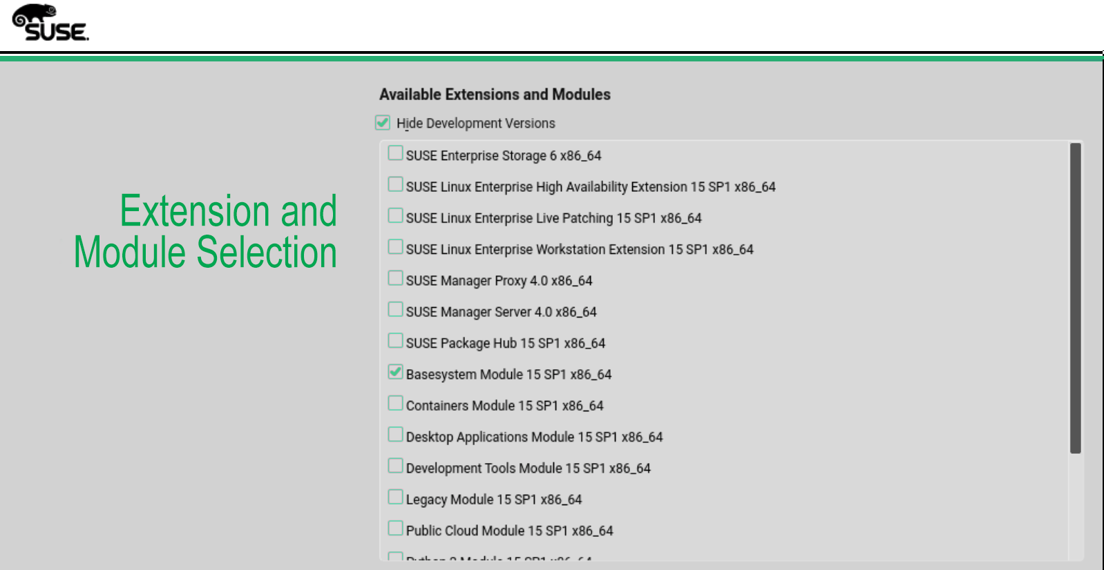
To simplify installation of NVIDIA CUDA Toolkit on SUSE Linux Enterprise for High Performance Computing (SLE HPC) 15, we have included a new SUSE Module, NVIDIA Compute Module 15. This Module adds the NVIDIA CUDA network repository to your SLE HPC system. You can select it at installation time or activate it post installation. This module is available for use with all SLE HPC 15 Service Packs.
Note that the NVIDIA Compute Module 15 is currently only available for the SLE HPC 15 product.
After YaST checks the registration for the system, a list of modules that are installed or available is displayed.
Click on the box to select the NVIDIA Compute Module 15 X86-64
Notice that a URL for the EULA is included in the Details section. Please comply with the NVIDIA EULA terms.
Information on the EULA for the CUDA drivers is displayed.
Agree and click Next
You must trust the GnuPG key for the CUDA repository.
Click Trust
You will be given one more confirmation screen
Click Accept
After adding the repository, you can install the CUDA drivers.
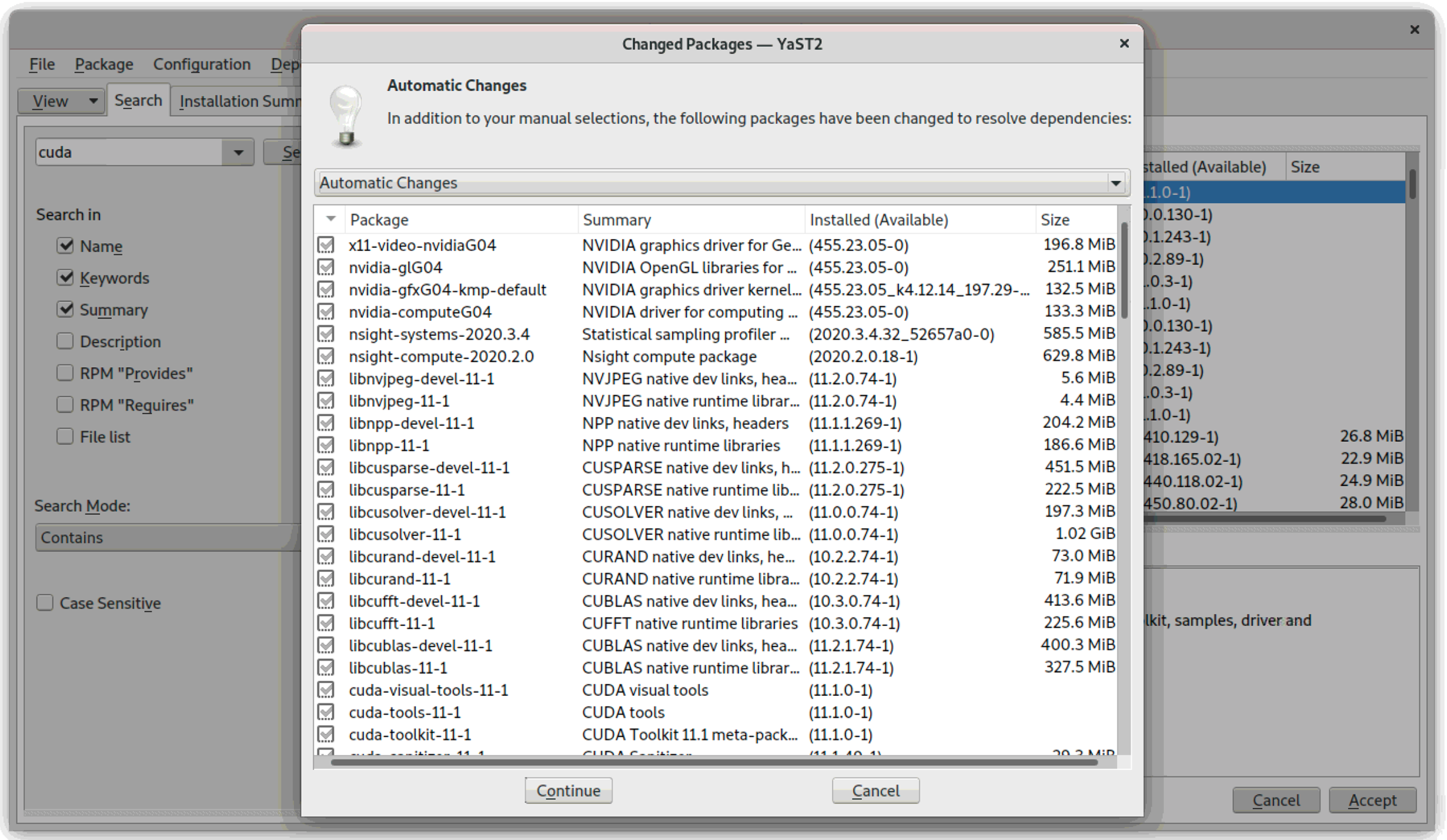
Start Yast and select Software Management” then search for cuda
Select the cuda meta package and press Accept
A large number of packages will be installed
Press Continue to proceed
That’s it!
You are now ready to start using the CUDA toolkit to harness the power of NVDIA GPUs.
Summry
Managing heterogeneous computing environments has become increasingly important for HPC and AI/ML administrators. The NVIDIA Compute Module is one way we are working to make using these technologies easier to use.
Since its introduction in 2006, Ceph has been used predominantly for volume-intensive use cases where performance is not the most critical aspect. Because the technology has many attractive capabilities, there has been a desire to extend the use of Ceph into areas such as High-Performance Computing. Ceph deployments in HPC environments are usually as an active archival (tier-2 storage) behind another parallel file system that is acting as the primary storage tier.
We have seen many significant enhancements in Ceph technology. Contributions to the open source project by SUSE and others has led to new features, considerably improved efficiency, and made it possible for Ceph-based software defined storage solutions to provide a complete end-to-end storage platform for an increasing number of workloads.
Traditionally, HPC data storage has been very specialised to achieve the required performance. With the recent improvements in Ceph software and hardware and in network technology, we now see the feasibility of using Ceph for tier-1 HPC storage.
The IO500 10-node benchmark is an opportunity for SUSE to showcase our production-ready software defined storage solutions. In contrast to some other higher ranked systems, this SUSE Enterprise Storage Ceph-based solution that we benchmarked was production-ready, with all security and data protection mechanisms in place.
This was a team effort with Arm, Ampere, Broadcom, Mellanox, Micron and SUSE to build a cost-effective, highly-performant system available for deployment.
The benchmark
The IO500 benchmark of IO performance combines scores for several bandwidth intensive and metadata intensive workloads to generate a composite score. This score is then used to rank various storage solutions. Note that the current IO500 benchmark does not account for cost or production readiness.
There are two lists for IO500 based upon the number of client nodes. The first list is for unlimited configurations and the second list is for what is termed the “10-node challenge”. ( More IO500 details) We chose the “10-node challenge” for this benchmark attempt.
Our previous benchmark was also for the 10-node challenge and it had a score of 12.43 on a cluster we called “Tigershark”. We created a new cluster this year, called “Hammerhead”, continuing with the shark theme.
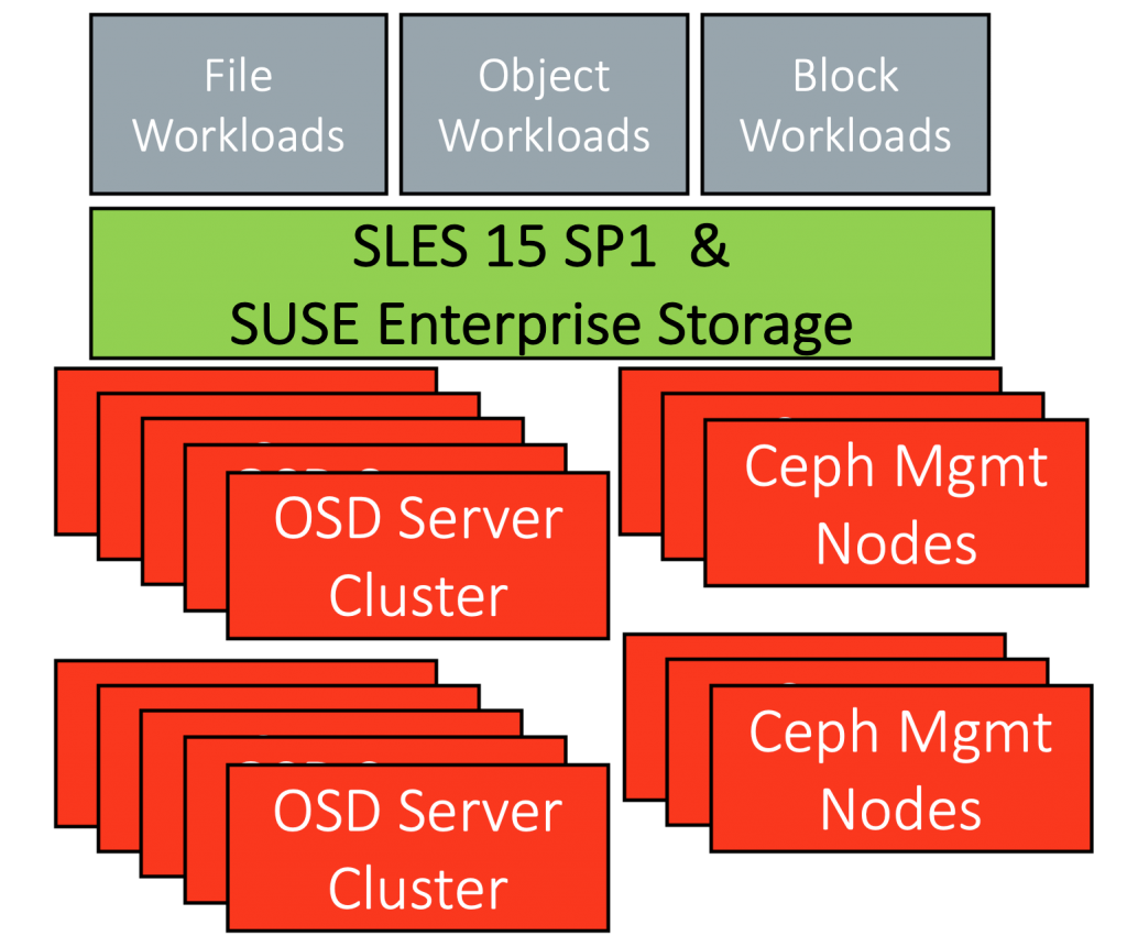
The solution
There have been no major updates to the software stack used for the 2019 IO500 benchmark. The operating system was SLES 15 Service Pack 1 with SUSE Enterprise Storage version 6, based on the Ceph version “Nautilus”.
Our goal was to beat our score from last year of 12.43 that was done (11/19 IO500 list) using an entirely different hardware platform and to validate the performance of an Arm-based server. We believe that any system we benchmark should emulate a production system that a customer may deploy, therefore all appropriate Ceph security and data protection features were enabled during the benchmark.
The hardware we used this year is substantially different even though it looks very similar. We used a Lenovo HR350A system, based on the Ampere Computing eMAG processor. The eMAG is a single socket 32 core ARM v8 architecture processor.
The benchmark was performed on a cluster of ten nodes as the data and metadata servers. Each server has 128GB of RAM and four Micron 7300PRO 3.84TB NVMe SSDs. These NVMe SSDs are designed for workloads that demand high throughput and low latency while staying within a capital and power consumption budget. Broadcom provided the HBA adapters in each storage node.
The cluster was interconnected with Mellanox’s Ethernet Storage Fabric (ENF) networking solution. The Mellanox technology provides a high-performance networking solution to eliminate data communication bottlenecks associated with transferring large amounts of data and is designed for easy scale-out deployments. ENF includes a ConnectX-6 100GbE NIC in each node connected by a SN3700 Spectrum 100GbE switch.
Network configuration is set up to use JUMBO frames with an MTU of 9000. We also increased the device buffers on the NIC and changed a number of sysctl parameters.
We used the tuned “throughput-performance” profile for all systems.
The last change was to alter the IO scheduler on each of the NVMEs and set it to “none”.
For the SUSE Enterprise Storage (SES) configuration, we deployed four OSD processes to each NVME device. This meant that each server was running with 16 OSD processes against four physical devices.
We ran a metadata service on every Arm node in the cluster which meant we had 12 active metadata services running.
We increased the number of PGs to 4096 for the metadata and data pools to ensure we had an even distribution of data. This is in line with the recommended number of PGs per OSD of between 50-100.
We also set the data protection of the pools to be 2X as we did in our last set of benchmarks. This is to make sure that any data that is written is protected.
As mentioned previously, we also left authentication turned on for the cluster to emulate what we would see in a production system.
The ceph.conf configuration used:
[global]
fsid = 4cdde39a-bbec-4ef2-bebb-00182a976f52
mon_initial_members = amp-mon1, amp-mon2, amp-mon3
mon_host = 172.16.227.62, 172.16.227.63, 172.16.227.61
auth_cluster_required = cephx
auth_service_required = cephx
auth_client_required = cephx
public_network = 172.16.227.0/24
cluster_network = 172.16.220.0/24
ms_bind_msgr2 = false

# enable old ceph health format in the json output. This fixes the
# ceph_exporter. This option will only stay until the prometheus plugin takes
# over
mon_health_preluminous_compat = true
mon health preluminous compat warning = false

rbd default features = 3

debug ms=0
debug mds=0
debug osd=0
debug optracker=0
debug auth=0
debug asok=0
debug bluestore=0
debug bluefs=0
debug bdev=0
debug kstore=0
debug rocksdb=0
debug eventtrace=0
debug default=0
debug rados=0
debug client=0
debug perfcounter=0
debug finisher=0

[osd]
osd_op_num_threads_per_shard = 4 prefer_deferred_size_ssd=0

[mds]
mds_cache_memory_limit = 21474836480  mds_log_max_segments = 256  mds_bal_split_bite = 4
The Results
This benchmark effort achieved a score of 15.6. This is the best CephFS IO500 benchmark on an Arm-based platform to date. This score was an improvement of 25% over last year’s results on the “Hammerhead” platform. The score put this configuration in the 27th place in the IO500 10-node challenge, two places above our previous benchmark.
During the benchmark, we saw that the Ceph client performance metrics could easily hit peaks in excess of 16GBytes/s for write performance with large file writes. Because we were using production-ready settings for 2X data protection policy, this means that the Ceph nodes were achieving 3GB/s I/O performance.
One of the most significant findings during this testing was the power consumption, or rather the lack of it. We used ipmitool to measure the power consumption on a 30 second average. The worst case 30 second average was only 152 watts, significantly less than we saw with last year’s benchmark.
In addition to the performance improvement and power savings, we believe this cluster would cost up to 40% less than last year’s configuration.
Conclusion
The purpose-built storage solutions used in HPC come at a significant cost. With the data volume increasing exponentially for HPC and AI/ML workloads, there is considerable pressure on IT departments to optimise their expenses. This benchmark demonstrates that storage solutions based on innovative software and hardware technology can provide additional choices for companies struggling to support the amount of data needed in HPC environments.
The partnership with Ampere, Arm, Broadcom, Mellanox, Micron and SUSE yielded a new, highly-performant, power efficient platform – a great storage solution for any business or institution seeking a cost-effective, low power alternative.
SUSE Linux Enterprise Server (SLES) 15 Service Pack 2 delivers support for new 64bit Arm processors and enhancements to previous Arm support. SUSE uses a “Refresh” and “Consolidation” approach to Service Pack releases: Every “Even” release (e.g., SP0, SP2,…) is a “Refresh” release that will include the latest stable Linux kernel. For SLES 15 SP2, we are using the 5.3 Linux kernel as the base with backports from later kernels as needed.
SUSE’s uses an “upstream first” approach to hardware enablement. That means that SUSE will not use “out of tree” or proprietary Board Support Packages is to enable new hardware, SUSE will only use drivers that has been enabled in upstream Linux. SUSE does work with the community to get new hardware support accepted upstream, but our “upstream first” approach reduces the risk of regression in a later Linux release.
Not all device drivers for new hardware is available upstream at the time SUSE ships a new release. In those cases, SUSE does as much enablement as possible in the current Service Pack, and implements additional drivers in later releases.
New Arm Systems on a chip (SoC) support in SP2*:
Ampere Altra
AWS Graviton2
Broadcom BCM2711 (for RPI 4)
Fujitsu A64FX
NXP LS1028A (no graphics driver available yet)
*Note: Please check with your specific hardware vendor regarding SUSE support for your specific server. Due to the rapidly evolution of Arm systems, not all Arm based servers have undergone the same degree of hardware testing.
New Arm servers enabled in SP2:
Raspberry Pi 4 (no accelerated graphics)
Raspberry Pi Compute Module 3B+
Raspberry Pi 3A+
NVIDIA TegraX1, NVIDIA TegraX2
Fujitsu FX700 (SUSE “YES” certified)
Other Arm enhancements
Support for up to 480 vCPU
Add rpi_cpufreq for Raspberry Pi to dynamically change frequency resulting in lower energy use and heat generation when idle
Add Arm V8.2 48-bit IPA for increased memory addressability
Enable Armv8.5 Speculation Barrier (SB) instruction to enhance security
Enable ARMv8.1-VHE: Virtualization Host Extensions for KVM optimization
Remove support for pre-production Marvell ThunderX2 processors
USB enabled for ipmitool to simplify flashing firmware on 64bit Arm systems such as HPE Apollo 70
Enable ARMv8.4 Unaligned atomic instructions and Single-copy atomicity of loads/stores
Improved U-Boot bootloader to support Btrfs filesystem offering additional flexibility for partitioning, scripting and recovery. (Tech-Preview)
Improved Installer experience on Raspberry Pi by ensuring all firmware, boot loader, and device tree packages are installed when using DVD media
QuickStart for Raspberry Pi updated
Last thoughts
There are a number of other encouraging events in the news about Arm servers:
These announcements underscore that Arm processor-based servers are finally starting to reaching critical mass for data center workloads. SUSE is proud to be part of the Arm server revolution.
SUSE Linux Enterprise for High Performance Computing (SLE HPC) 15 Service Pack 2 has a lot of new capabilities for HPC on-premises and in the Cloud.
SUSE uses a “Refresh” and “Consolidation” approach to Service Pack releases: Every “Even” release (e.g., SP0, SP2, …) is a “Refresh” release that will include the latest stable Linux kernel. For SLES 15 SP2, we are using the 5.3 Linux kernel as the base with backports from later kernels as needed. Updating to a new kernel every two releases allows SUSE to provide our customers with the Linux features and enhancements.
SUSE Linux Enterprise for HPC
When we introduced the HPC Module to SUSE Linux early in 2017, we laid out a strategy to make High Performance Computing adoption easier by providing a several fully supported HPC packages to our SUSE Linux customers.
These packages have been built and tested by SUSE and are provided at no additional cost with the SUSE Linux support subscription.
SUSE provides the HPC Module for customers using the X86-64 and Arm hardware platform. Except for a few hardware specific packages, all the packages are supported on both platforms. If you haven’t tried the HPC module yet, here are the instructions on how to access it. The HPC Module is also included in HPC images available on Clouds like Microsoft Azure.
HPC Module updates
Added adios1.13.1
boost to 1.71.0
conman to version 0.3.0
cpuid to version 20180519
fftw3 to version 3.3.8
genders to version 1.27.3
gsl to version 2.6
hdf5 to version 1.10.5
hwloc to version 2.1.0
hypre to version 2.18.2
imb to version 2019.3
luafilesystem to version 1.7.0
lua-lmod to version 8.2.5
lua-luaposix to version 34.1.1
memkind to version 1.9.0
mpich to 3.3.2
mvapich2 to version 2.3.3
mumps to version 5.2.1
netcdf to version 4.7.3
netcdf-cxx4 to version 4.3.1
netcdf-fortran to 4.5.2
python-numpy to version 1.17.3
python-scipy to version 1.3.3
openblas to 0.3.7
Added openmpi3 3.1.4
papi to version 5.7.0
petsc to version 3.12.2
Added PMIx version 3.1.5
scalapack to 2.1
scotch to version 6.0.9
slurm to 20.0.2
trilinos to version 12.14.1
HPC relevant base system packages
libfabric 1.8 to enable AWS
rdma-core 24.0 to enable AWS
PackageHub
PackageHub is a SUSE curated repository for community supported, open-source packages. A number of AI/ML packages were added to PackageHub for SP2. These packages can be installed using zypper. Tips for using PackageHub.
armnn 20.02
caffe 1.0
charliecloud 0.15
clustershell 1.8.2
numpy 1.17.3
pytorch
robinhood 3.1.5
singularity 3.5.2
tensorflow2 2.1.0
theano 1.0.4
warewolf 3.8.1
New HPC and ML/AI Systems
SLE HPC 15 SP2 enabled a number of servers for HPC and AI/ML workloads including:
NVIDIA TegraX1
NVIDIA TegraX2
Fujitsu FX700 – (also SUSE “YES” certified)
AWS Graviton2 instances in AWS Cloud
Other HPC changes
Add Elastic Fabric Adapter (EFA) driver to enable HPC on AWS
Add the Live Patching Extension to the SLE-HPC Product
Improve clustduct cluster distribution tool
Remove unneeded package ‘ohpc’
Summary
The HPC ecosystem continues to expand and transform to include simulation, data analytics, and machine learning. SUSE HPC will continue to grow with the needs of our customers.
SUSE recently updated Terms and Conditions for SUSE products to clarify the SUSE pricing policies for IBM Power systems and to accommodate Sub-capacity pricing on IBM Power servers.
Sub-capacity pricing overview
IBM Power servers have long been known for vertical scalability (up to 192 cores and 64TB of RAM) and for efficient PowerVM virtualization infrastructure. As a result, many customers use IBM Power servers to consolidate multiple workloads on a single server.
PowerVM virtualization can guarantee that a particular workload can only run on a subset of the processors on a particular system. For example, you could have a 192 core IBM Power server with 32 cores running a DB2 database with AIX and the other 160 cores could be running SAP HANA on SUSE Linux for SAP Applications.
Software subscriptions traditionally have been priced based on the amount of CPU capacity available to run the software, fewer cores generally mean lower software cost. This is known as Sub-capacity pricing because the customer is only paying for software based on a subset of the total hardware capacity.
Most IBM software is sold based on Sub-capacity pricing, so IBM Power customers expect to pay for software licenses or subscriptions based on the amount of processor capacity available to each workload.
Sub-capacity pricing for SUSE products on IBM Power
SUSE products started on X86 servers, where prices were traditionally based on the number of processor sockets as a measure of CPU capacity. Server consolidation is less prevalent in the X86 market and Sub-capacity pricing for software is less common. As a result, the price of most SUSE subscriptions is based on the number of processor sockets available in the server, known as Full-capacity pricing.
In view of the unique capabilities of the IBM Power platform, we have changed the Terms and Conditions for SUSE product subscriptions to accommodate Sub-capacity pricing on Power. This will allow customers to partition their IBM Power servers with PowerVM virtualization and only pay for the capacity available to that SUSE product on a particular server.
The charge metric of SUSE product subscriptions on IBM Power has not been changed and is still measured in “socket pairs”. Because IBM PowerVM allocates processor capacity in terms of processor cores, there needs to be a way to convert the “cores” allocation in PowerVM to the equivalent number of socket pairs for SUSE subscription purposes.
Because SUSE subscriptions are sold in increments of socket pairs, to use Sub-capacity pricing on Power while still using socket pairs, you need to calculate the Socket Pair Equivalent that represents the CPU capacity that is made available to the SUSE workload.
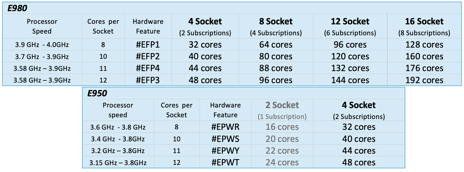
Unfortunately, there is another complication in that IBM Power servers have different numbers of cores per socket, and thus per socket pair. For example, an IBM E980 server with hardware feature #EFP1 has 8 cores per socket, or 16 cores per socket pair. The same hardware ordered with feature #EFP3 has 12 cores per socket or 24 cores per socket pair. You must know the number of cores per socket in the server before you can calculate the Socket Pair Equivalent for SUSE subscription purposes. The number of cores per socket on an IBM Power server is tied to the processor speed. Faster speed = Fewer cores per socket.
Conditions for using Sub-capacity pricing for SUSE products on IBM Power
The SUSE product must use socket pairs as the charge metric.
SUSE Linux Enterprise Server (SLES) for Power, SLES for SAP Applications on Power, SUSE Manager Server for Power and SUSE Manager Lifecycle for Power are all included.
This is only applicable to POWER8 and POWER9 (and later generations) with four or more sockets.
E850, E880, E870, E950, and E980 are all eligible for Sub-capacity pricing.
PowerVM virtualization must be used to restrict the amount of capacity available to the SUSE products being used
Acceptable methodologies: Dedicated processor partitions (Dedicated LPAR), Dynamic LPAR, Single or Multiple Shared Processor Pools
The Integrated Facility for Linux (IFL) processors does not automatically limit Linux workloads to only run on IFL processors and are not relevant to Sub-capacity pricing.
Customers and Sellers must account for the different number of cores per socket when calculating the Socket Pair Equivalent
Number of cores available to SUSE Linux ÷ by the number of cores per socket = Socket Pair Equivalent
Round up to nearest socket pair
The customer must purchase subscriptions for the maximum number of socket pairs that are ever available to run SUSE workloads.
Customer is responsible for purchasing additional subscriptions if the processor capacity is increased through changes to pools or activation of dark processors or other changes to the server capacity.
Example 1: Calculating Socket Pair Equivalent for IBM Power E950
In this example, the E950 has 10 cores per socket = 20 cores per socket pair.
Example 2: Calculating Socket Pair Equivalent for IBM Power E950 with Rounding
In this example, the E950 has 10 cores per socket = 20 cores per socket pair.
You can see that if the calculations end up with a fractional value, (that is, the number of cores is not an integer number of sockets) you must round up to the next nearest integer.
Example 3: Calculating Socket Pair Equivalent for IBM Power E950 lower core count and rounding
In this example, the E950 has 8 cores per socket = 16 cores per socket pair.
As in the previous example, you can see that if the calculations end up with a fractional value, (that is, the number of cores is not an integer number of sockets) you must round up to the next nearest integer.
Example 4: Calculating Socket Pair Equivalent for IBM Power E950 with Dynamic LPAR
In this example, the E950 has 10 cores per socket = 20 cores per socket pair and the system administrator is using Dynamic LPAR (DLPAR) to dynamically change the number of cores available to SLES for SAP.
Before the DLPAR operation, the SLES for SAP LPAR/VM had 18 cores of capacity which would round up to 1 socket pair of capacity but after the DLPAR operation, the SLES for SAP LPAR/VM is over 2 sockets of capacity and thus requires 2 SLES for SAP subscriptions.
The customer must provide enough SUSE subscriptions to cover the maximum capacity ever used.
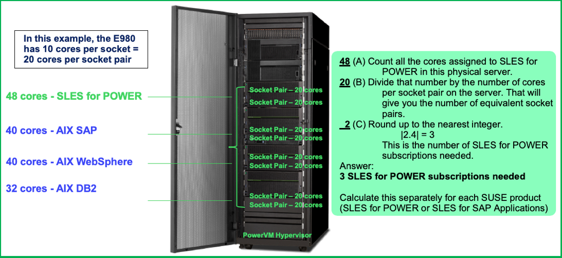
Example 5: Calculating Socket Pair Equivalent for IBM Power E980 Server Consolidation
In this example, the E980 has 10 cores per socket = 20 cores per socket pair.
Once again, we see that if the number of cores assigned to the SUSE product is more than 2 socket pairs, so 3 SLES for Power subscriptions are needed for this configuration.
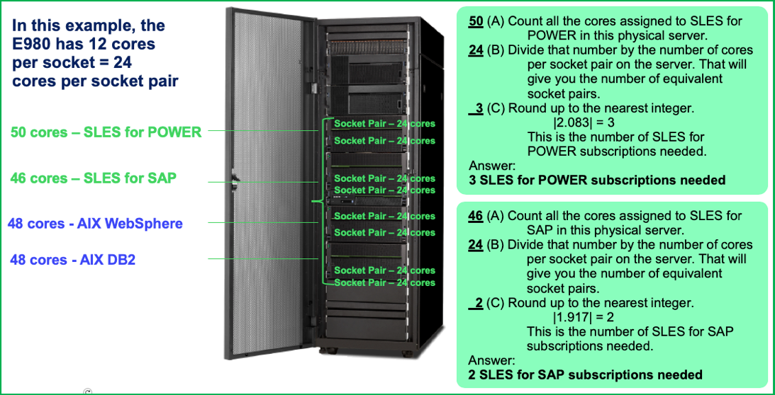
Example 6: Calculating Socket Pair Equivalent for IBM Power E980 with multiple SUSE products
In this example, the E980 has 12 cores per socket = 24 cores per socket pair.
There are two different SUSE products installed on this system. The Socket Pair Equivalent calculation must be performed for each SUSE product installed on a physical server.
Summary
Server consolidation is a common practice for IBM Power servers and Sub-capacity pricing is important to supporting consolidation. Using the Socket Pair Equivalent approach allows customers to leverage Sub-capacity pricing for SUSE products on IBM Power servers and to leverage the capabilities of PowerVM while maintaining compliance with SUSE terms and conditions.
Reference: Cores / Socket for IBM POWER9 Enterprise servers
Reference: Cores / Socket for IBM POWER8 Enterprise servers
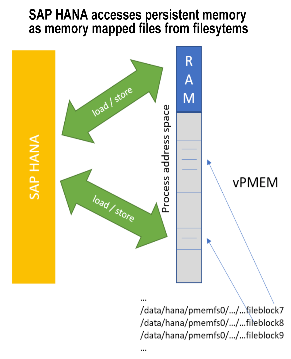
SAP HANA uses in-memory database technology that allows much faster access to data than was ever possible with hard disk technology on a conventional database – access times of 5 nanoseconds versus 5 milliseconds. SAP HANA customers can also use the same database for real-time analysis and decision-making that is used for transaction processing.
The combination of faster access speeds and better access for analytics has resulted in strong customer demand for SAP HANA. There are already more than 1600 customers using SAP HANA on Power since it became available in 2015.
One of the drawbacks of in-memory databases is the amount of time required to load the data from disk into memory after a restart. In one test with an 8TB data file representing 16TB database, it took only six minutes to shut down SAP HANA, but took over 40 minutes to completely load that database back into memory. Although the system was up and responsive much more quickly, it took a long time for all data to be staged back into memory.
SAP has implemented features such as the Fast Restart Option to reduce the database load time, but system providers have enhancements to help address the problem. Intel introduced Optane DC memory technology where the data in memory is preserved even when powered down. Optane DC is positioned as a new tier of storage between DRAM and flash storage with more capacity at a lower price than DRAM but with less performance. Optane DC memory can deliver very fast restarts of SAP HANA but introduces new operational management complexity associated with adding a fourth tier of storage.
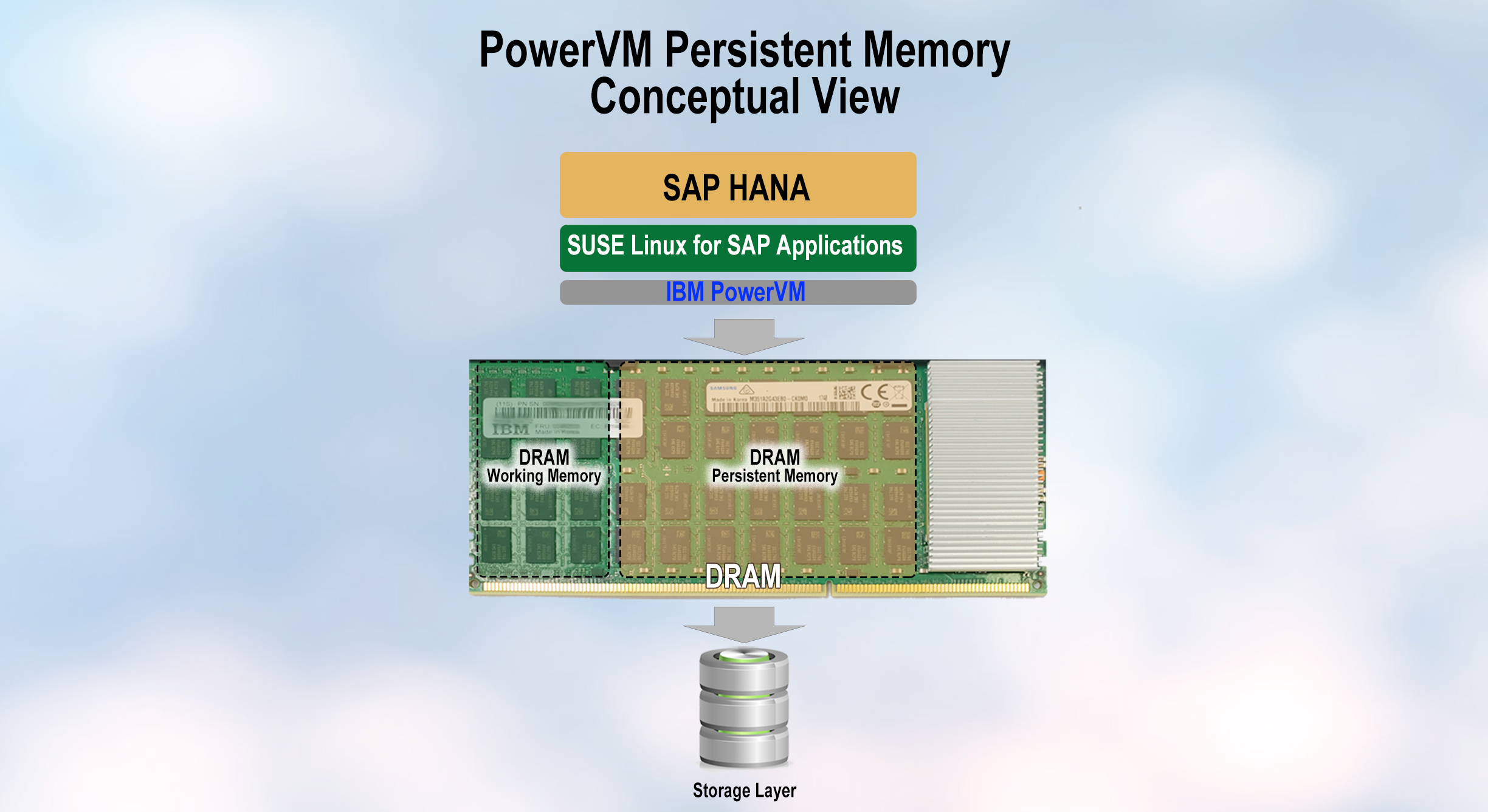
IBM PowerVM Virtual Persistent Memory
In October 2019, IBM announced Virtual Persistent Memory (vPMEM) with PowerVM. Virtual Persistent Memory isn’t a new type of physical memory but is a way to use the PowerVM hypervisor to create persistent memory volumes out of the DRAM that is already installed on the system. vPMEM is included at no additional charge with PowerVM.
The data in memory is persistent as long as the physical Power server is not powered off. By maintaining data persistence across application and partition restarts, it allows customers to leverage fast restart of a workload using persistent memory. An added benefit is that there is no difference in application performance when using vPMEM because the underlying DRAM technology is the same as for the non-persistent memory.
Although vPMEM does not preserve memory across a server power down, most IBM Power customers seldom power off their systems because of the many reliability features that are built into Power hardware. vPMEM provides for fast restart in the vast majority of planned maintenance and unplanned outages without compromising the performance of HANA during normal use.
Prerequisites
vPMEM has several prerequisites:
POWER9 processor-based systems
Hardware Management Console (HMC) V9R1 M940 or later
SUSE has three technical support bulletins that you should review before implementing vPMEM
TID 7024333 “Activation of multiple namespaces simultaneously may lead to an activation failure”
TID 7024330 “vPMEM memory backed namespaces configured as a dump target for kdump/fadump takes a long time to save dump files”
TID 7024300 “Hot plugging/unplugging of pmem memory having a size that is not in multiples of a specific size can lead to kernel panics”
Summery
Virtual Persistent Memory is the latest tool in a long line of IBM and SUSE innovations to help customers get the most out of their SAP HANA on Power environments.
You should strongly consider using vPMEM when running SAP HANA on POWER9 systems.
If you are new to SUSE Linux, you might have wondered why the C compiler on the system is so old. For example, on a SUSE Linux Enterprise Server (SLES) 12 Service Pack (SP) 3 system running on X86-64, the default gcc is version 4.8-6.189! Why isn’t the C compiler a newer version, like gcc version 8?
A SUSE Linux system can have multiple versions of the gcc compiler. The first type of compiler, the one used to compile the version of SUSE Linux that you are running, is known as the “System Compiler”. The “System Compiler” usually does not change throughout the life of the SLES version because changing it would greatly complicate creating patches to maintain the operating system. For example, gcc 4.8 is the SLES 12 “System Compiler” used to compile all SLES 12 releases including all Service Packs. gcc 7-3.3.22 is the “System Compiler” for SLES 15.
The other type of compilers available on SLES are known as a “Toolchain Compilers”. These are the primary compilers for application development and are periodically updated with patches and new stable compiler versions as they become available. Usually there is more than one version available at any point in time. Most developers want to use newer compilers for application development because they provide additional optimization and functionality.
Installing the newer “Toolchain” compilers is easy, but first you must understand a little about the SUSE Linux Modules concept.
SUSE Linux Modules Introduction
SUSE introduced the concept of operating system Modules in SLES 12. SLES Modules are groups of packages with similar use cases and support status that are grouped together into a Module and delivered via a unique repository. SUSE introduced the Module concept to allow delivery of the latest technology in areas of rapid innovation without having to wait for the next SLES Service Pack. SUSE fully maintains and supports the Modules through your SUSE Linux subscription.
With the introduction of SLES 15, Modules have become even more important because the entire SUSE Linux OS is packaged as modules. The SLES 15 installation media consists of a unified Installer and a minimal system for deploying, updating, and registering SUSE Linux Enterprise Server or other SUSE products. Even the ls and ps commands are part of “Basesystem Module 15” module in SLES 15.
During deployment you can add functionality by selecting modules and extensions to be installed. The availability of certain modules or extensions depends on the product you chose in the first step of this installation. For example, in SLES 15, the HPC Module is only available if you selected the SUSE Linux Enterprise for HPC product during the initial installation.
SUSE Linux Modules enable you to install just the set of packages required for the machine’s purpose, making the system lean, fast, and more secure. This modular packaging approach also makes it easy to provide tailor-made images for container and cloud environments. Modules can be added or removed at any time during the lifecycle of the system, allowing you to easily adjust the system to changing requirements. See the Modules Quick Start Guide for more information.
Please note that just activating a Module does not install the packages from that Module—you need to do that separately after activating a Module. To use a package from a Module generally requires two steps: 1) activating the Module and 2) installing the desired packages. Some Modules are pre-activated based on the product you installed. For example, the HPC Module is automatically activated when you install SUSE Linux for High Performance Computing 15.
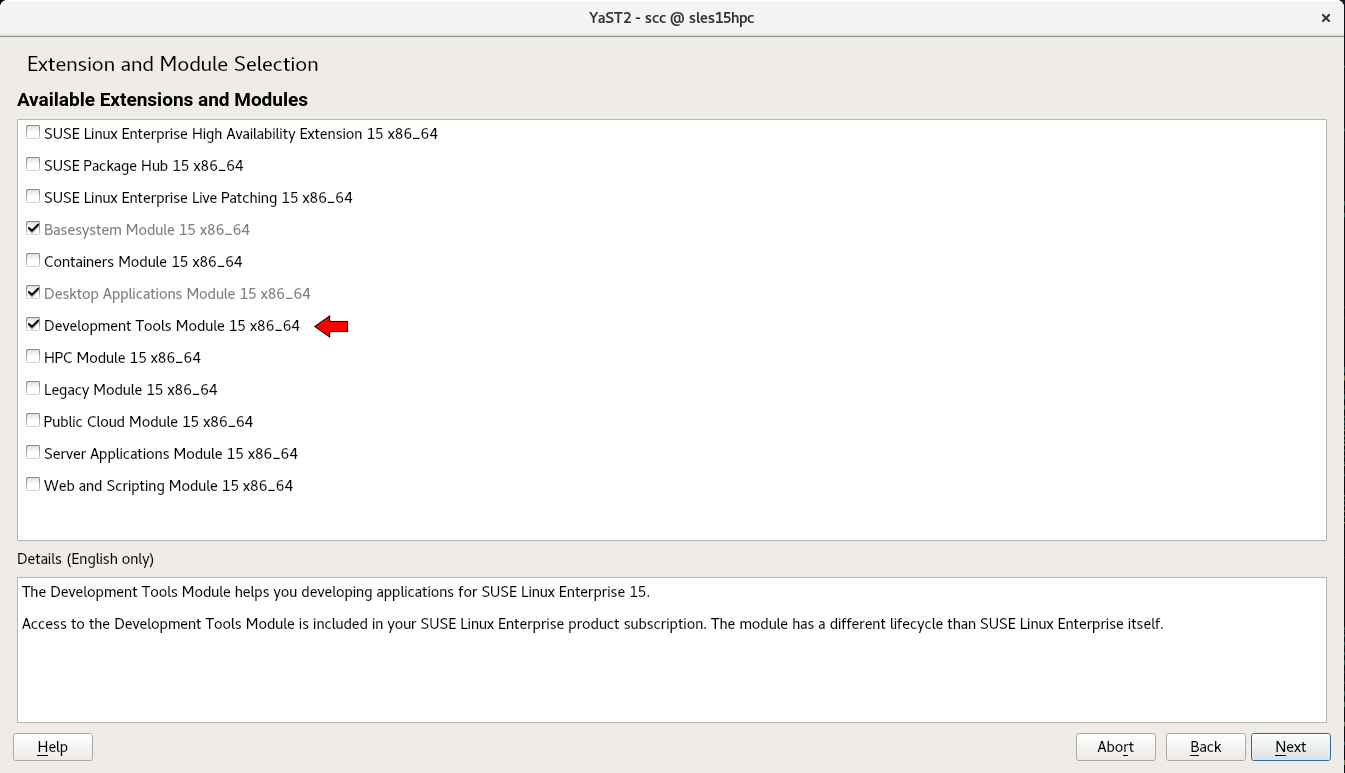
The Development Tools Module is the SLES 15 Module that includes the most recent compilers such as gcc, debuggers, and other development tools (over 500 packages for SLES 15). The Toolchain Module provided access to newer compilers for SLES 12.
Activating the Development Tools Module using YaST
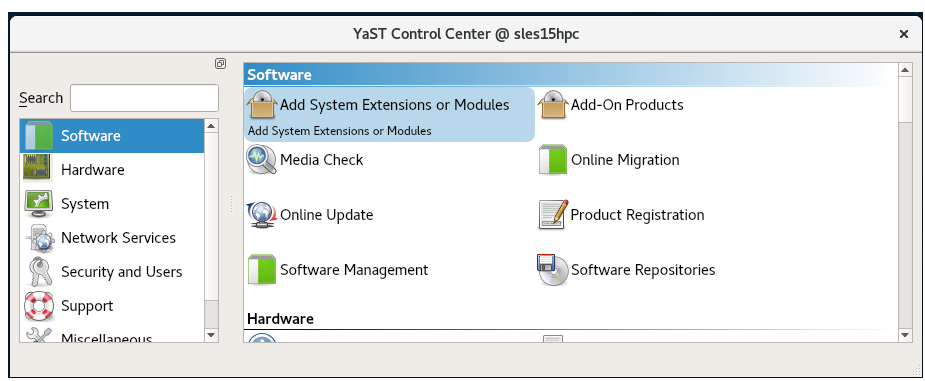
Start YaST. # Requires root privileges
Click Add System Extensions or Modules.
Select Development Tools Module.
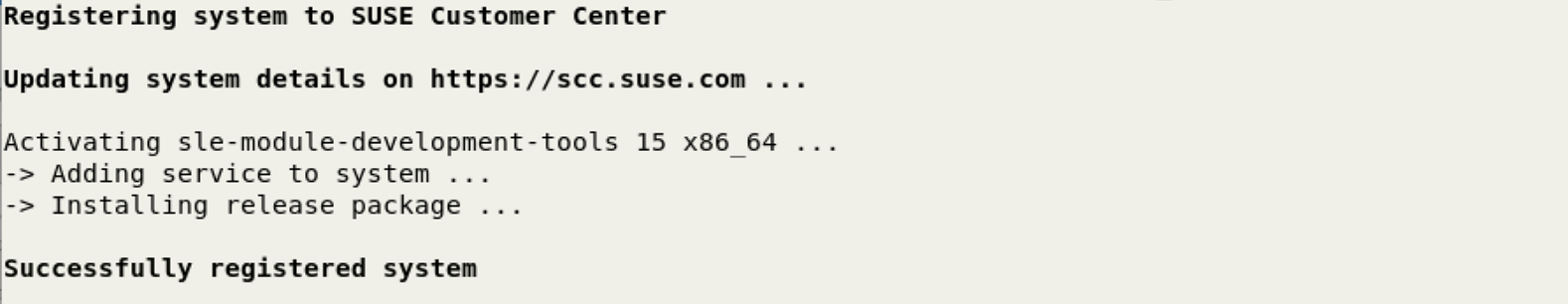
Press Next to start the activation process for the Development Tools Module
Installing a package (gcc8) from the Development Tools Module
Once the Development Tools Module is activated, you can install packages from the Module. This example uses gcc8.
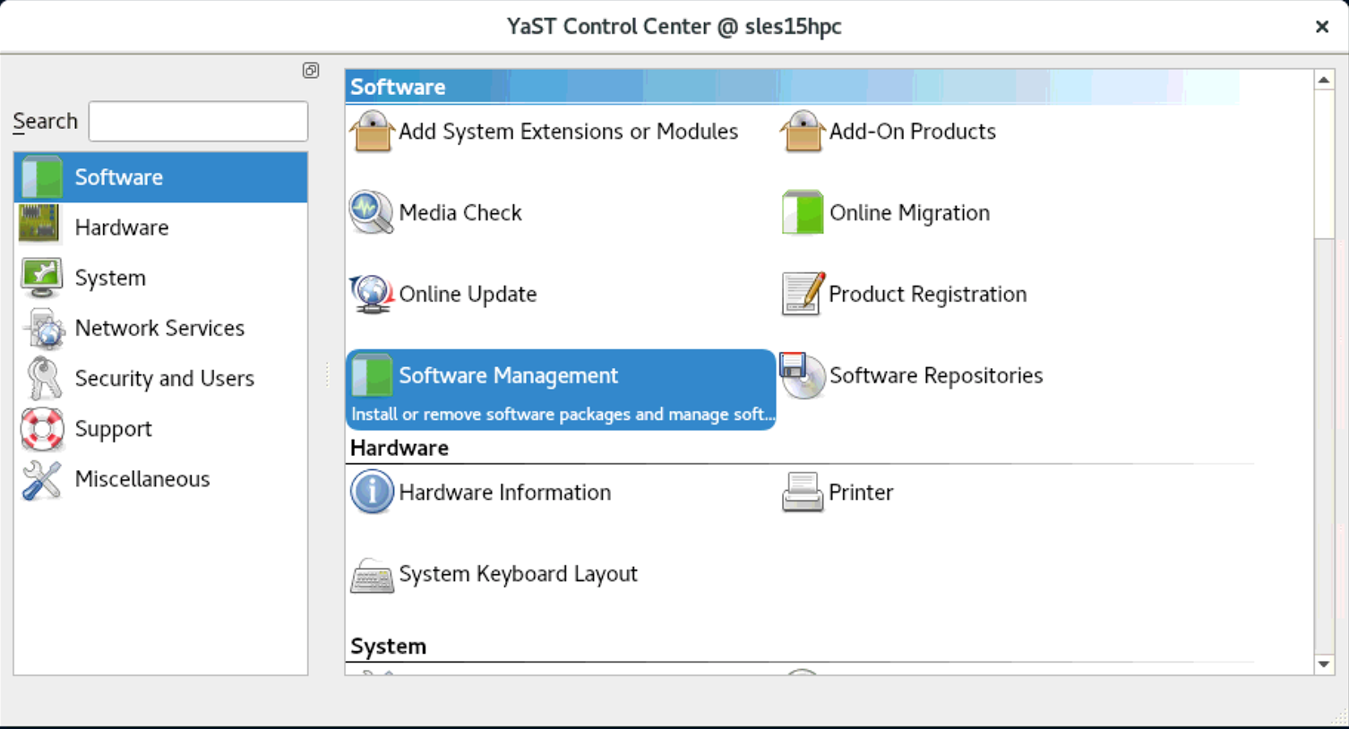
Start YaST and click Software then Software management
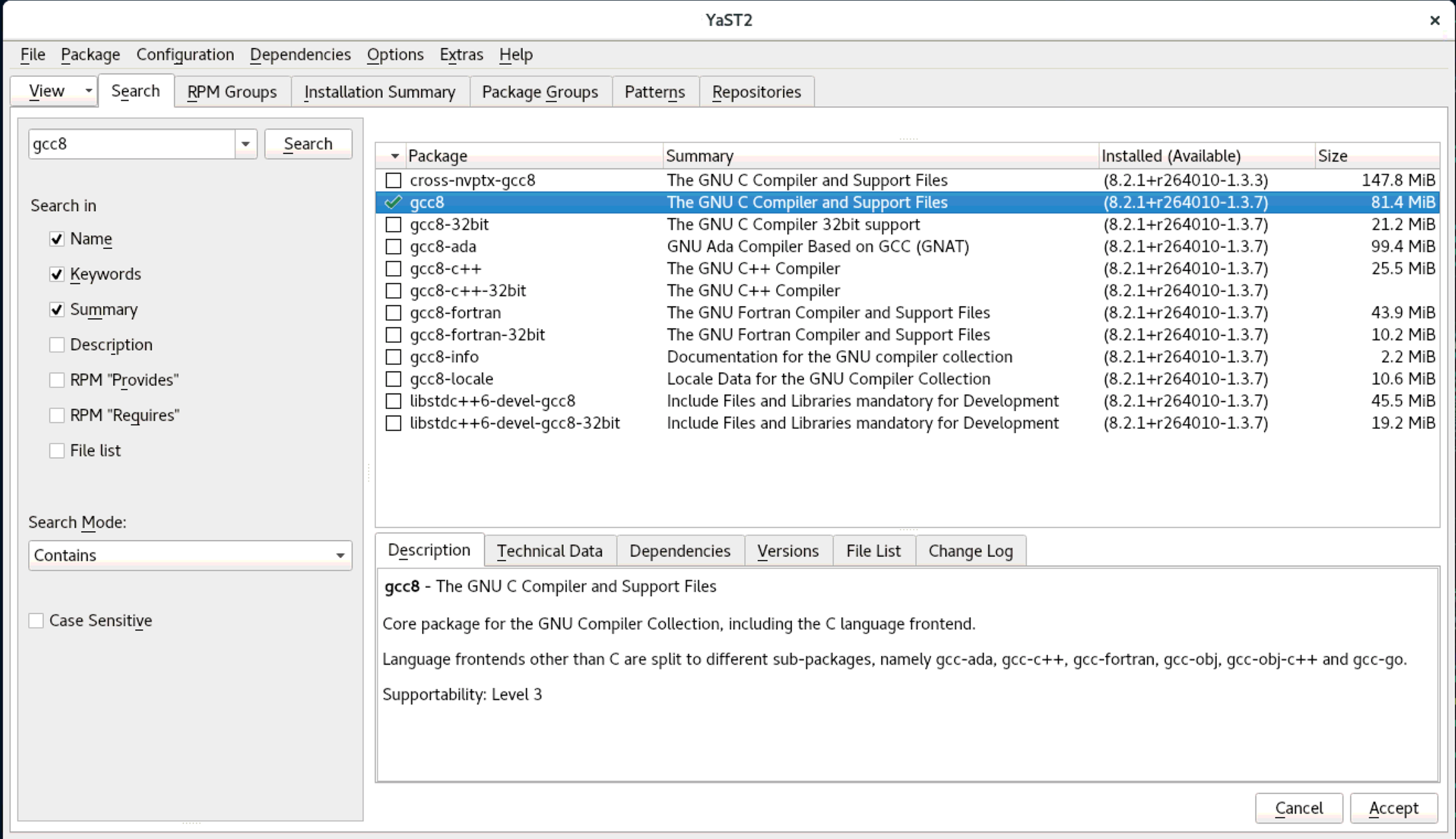
Type gcc8 in the search field and click Search.
Select gcc8 and click Accept.
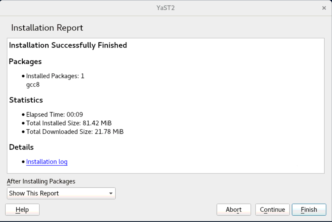
The gcc8 compiler will now be installed.
And that’s it! You have successfully activated the Development Tools Module and installed gcc8.
Activating the Development Tools Module on SLES 15 using the command line
Now let’s take a different approach and use the command line to perform the same tasks. You will need to have root privileges to perform most of these steps either by su to root or using sudo.
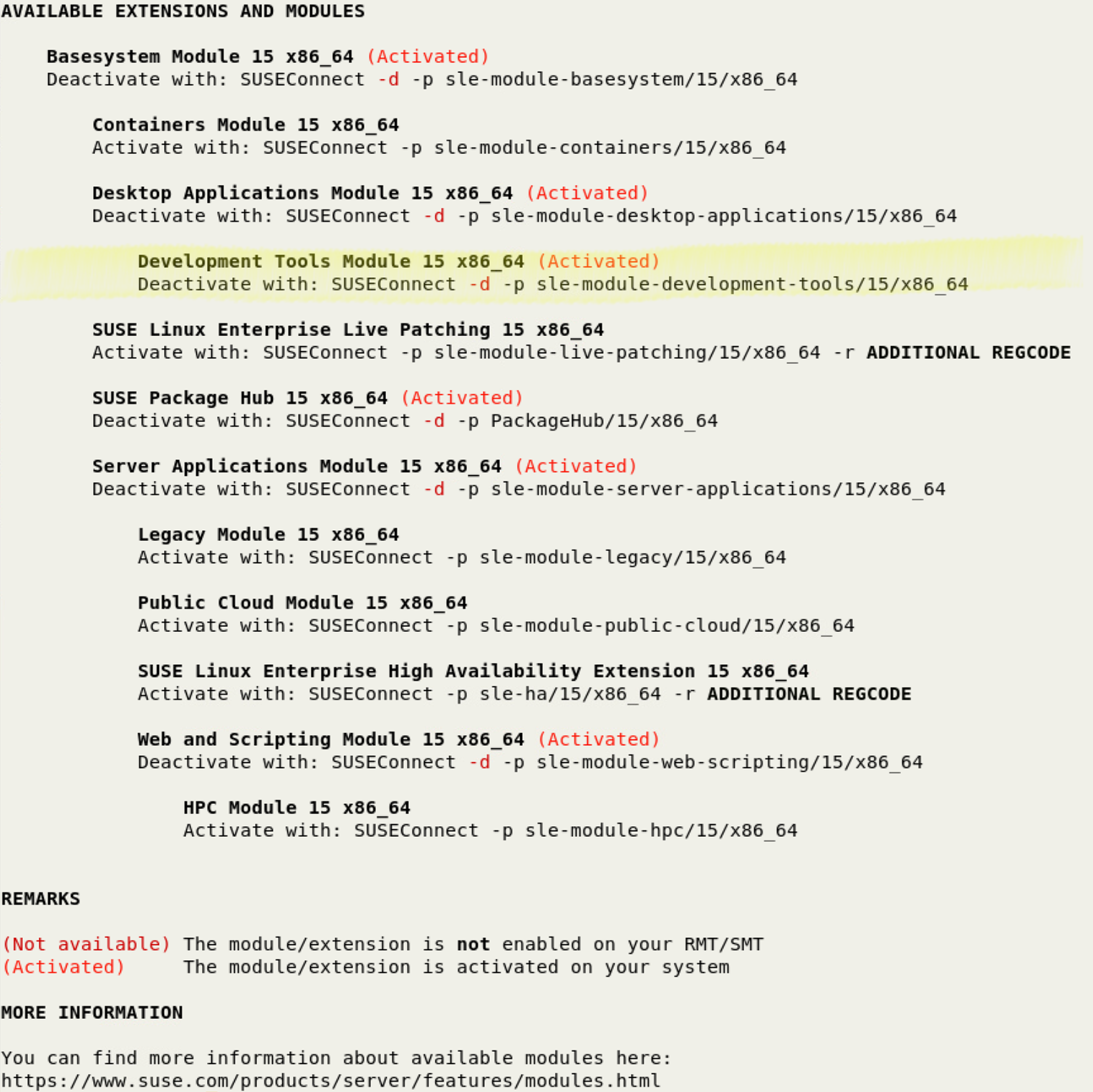
Verify that the Development Tools Module is activated.
sudo SUSEConnect –l
In this example, the BaseSystem, Development Tools, Desktop Applications, and Web and Scripting Modules are activated. The other Modules and Extensions are available for activation.
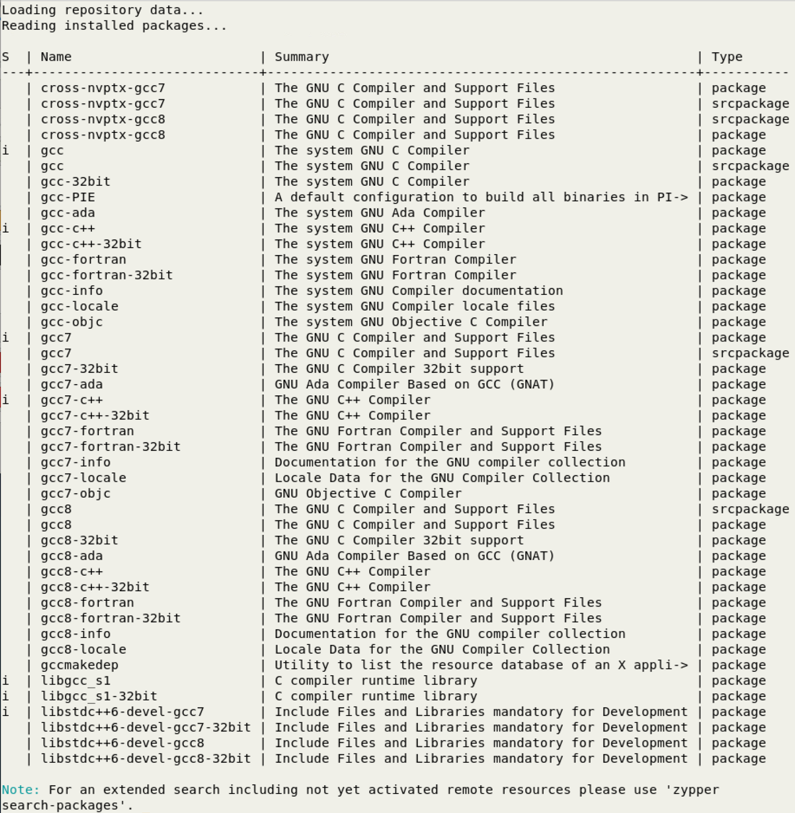
Check the status of gcc on this system.
zypper search gcc
You can see that the system C compiler is gcc7 and is installed (i) and gcc8 is available for installation.
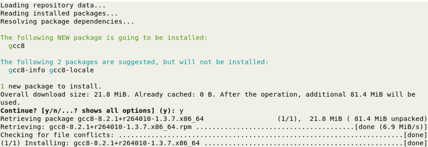
Install the gcc8 compiler.
sudo zypper install gcc8 # Must be root
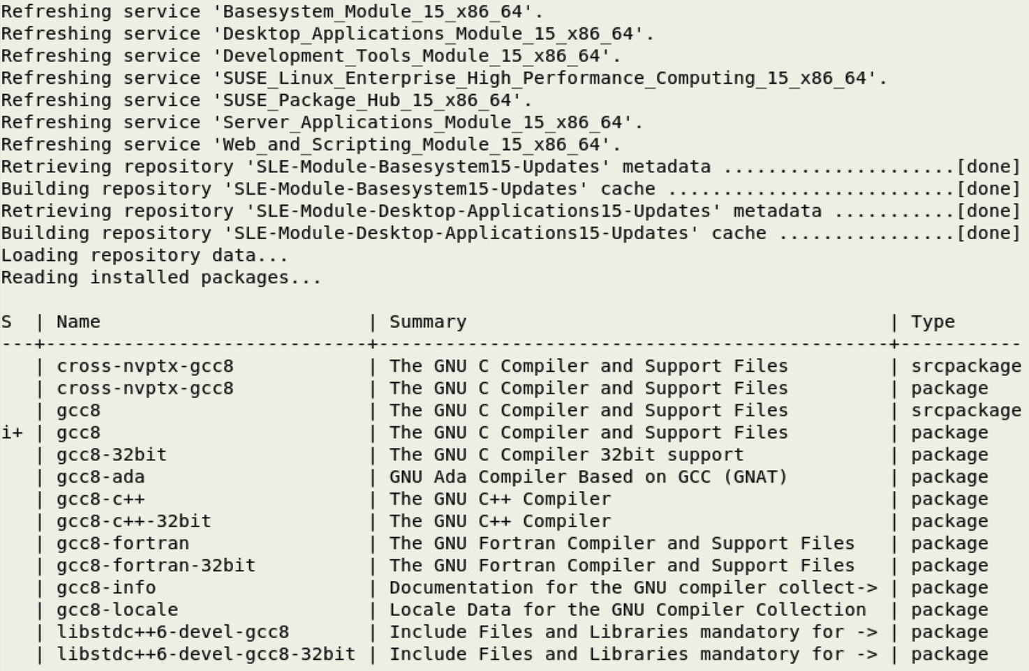
Verify that the gcc8 compiler was installed
zypper search gcc8
Check the gcc8 version.
gcc-8 –version
Summary
You should now understand how to activate a SUSE Module and install a package from the module. This same approach can be applied to the other SUSE Modules, such as the HPC Module. Modules are a key concept of SUSE product packaging, particularly for SLES 15.


 SUSE Linux Enterprise Server (SLES) 15 Service Pack 2 delivers support for new 64bit Arm processors and enhancements to previous Arm support. SUSE uses a “Refresh” and “Consolidation” approach to Service Pack releases: Every “Even” release (e.g., SP0, SP2,…) is a “Refresh” release that will include the latest stable Linux kernel. For SLES 15 SP2, we are using the 5.3 Linux kernel as the base with backports from later kernels as needed.